FCUP

• FCUP
• Define the Model
• Define the seeds
• Compute the streamlines
• plot the streamlines
• Compute the connections

This is a more advanced tutorial because we want to show how to apply a mask.

Define the Model

import Tractography as TG

model = TG.Model(Δt = 0.125f0,
            foddata = TG.FODData((@__DIR__) * "/../../examples/fod-FC.nii.gz"),
            cone = TG.Cone(45),
            proba_min = 0.015f0,
            )

Model with elype Float32
 ├─ Δt = 0.125
 ├─ minimal probability     = 0.015
 ├─ cone                    = Cone{Int64}(45)
 ├─ mollifier               = max_mollifier
 ├─ evaluation of the basis = PreComputeAllFOD()
 └─ data : (lmax = 8)

Just for fun, we plot the FODs of the model.

using CairoMakie

f, sc = TG.plot_fod(model; n_sphere = 1500, radius = 0.3, st = 2);
cam3d = Makie.cameracontrols(sc)
cam3d.eyeposition[] = Vec3f(85, 95, -28)
cam3d.lookat[] = Vec3f(84, 95, 59)
rotate_cam!(sc.scene, 0, 0, -pi/2)
f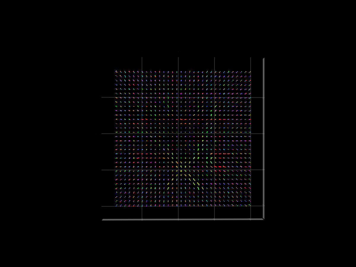

Define the seeds

We next apply a mask on the boundary of which the streamlines stop.

using NIfTI
mask = NIfTI.niread((@__DIR__) * "/../../examples/wm-FC.nii.gz");
TG._apply_mask!(model, mask);

┌ Warning: #= line 0 =#:
│ `LoopVectorization.check_args` on your inputs failed; running fallback `@inbounds @fastmath` loop instead.
│ Use `warn_check_args=false`, e.g. `@turbo warn_check_args=false ...`, to disable this warning.
└ @ LoopVectorization ~/.julia/packages/LoopVectorization/Y0o9B/src/condense_loopset.jl:1166

We compute Nmc streamlines, hence we need Nmc seeds

Nmc = 100_000
seeds = TG.from_fod(model, Nmc; maxfod_start = true)

6×100000 Matrix{Float32}:
  68.9081    122.867      60.0415    …  87.4581    129.142      44.5605
 120.385     119.802      54.0295       45.133      68.582      74.9766
   9.47406     3.4619      9.44593       6.20572     2.77065     8.77504
   0.914702   -0.984924    0.802262     -0.719292   -0.994637    0.989012
   0.393045   -0.0958604  -0.385279     -0.691566    0.0171193  -0.0579627
  -0.094      -0.144      -0.456     …   0.066       0.102       0.136

Compute the streamlines

streamlines, tract_length = TG.sample(model, TG.Deterministic(), seeds; nt = 1000);
println("Dimension of computed streamlines = ", size(streamlines))

kernel : 6.827028 seconds (916.79 k allocations: 44.523 MiB, 4.00% compilation time)
Dimension of computed streamlines = (3, 1000, 100000)

plot the streamlines

f, scene = @time TG.plot_fod(model; n_sphere = 500, radius = 0.3, st = 1);
ind_st = findall(tract_length .> 60)
TG.plot_streamlines!(scene, streamlines[:, :, ind_st[1:10:end]])
f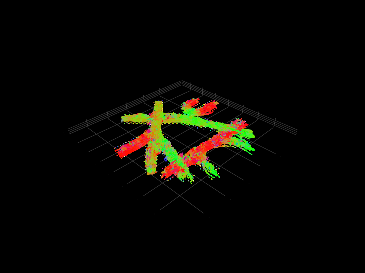

We can also add the seeds

scatter!(scene, seeds[1:3, ind_st[1:10:end]], color = :white)
f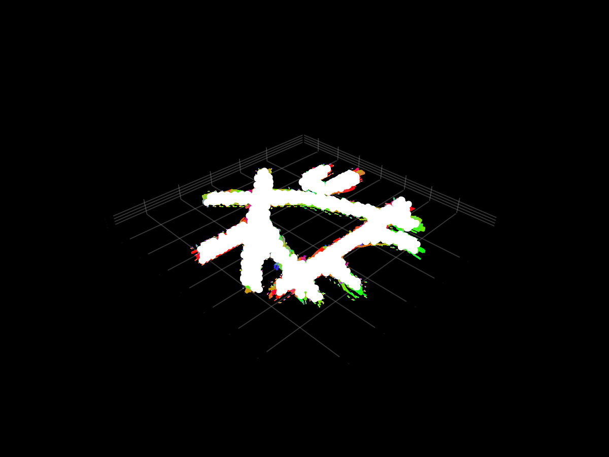

Compute the connections

When computing structural connectivity, we don't need to record the entire streamline but only its extremities.

streamlines, tract_length = TG.sample(model, TG.Connectivity(TG.Deterministic()), seeds; nt = 1000);
println("Dimension of computed streamlines = ", size(streamlines))

kernel : 6.554337 seconds (291.14 k allocations: 13.811 MiB, 2.67% compilation time)
Dimension of computed streamlines = (3, 2, 100000)